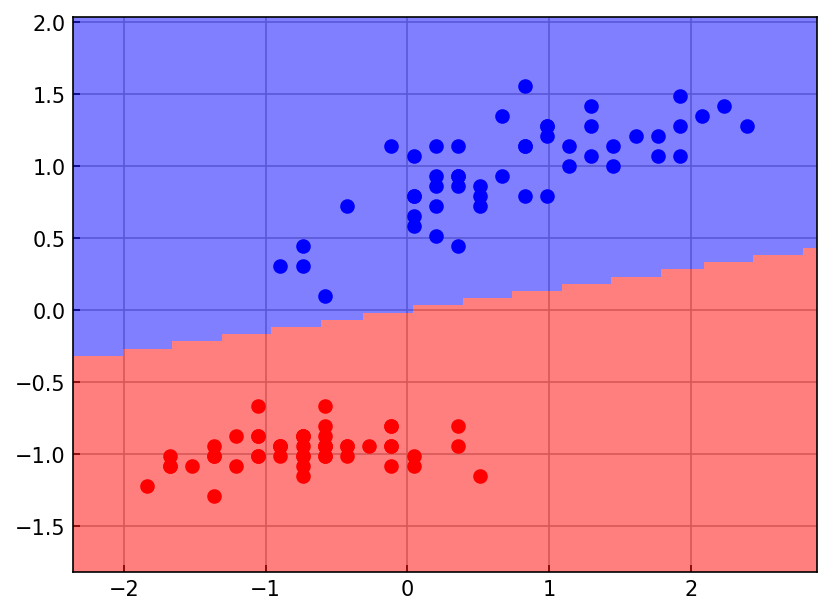
Adaptive Linear Neuron (Adaline)
%matplotlib inline

import numpy as np
import matplotlib.pyplot as plt

plt.rcParams['xtick.direction'] = 'in'
plt.rcParams['ytick.direction'] = 'in'
plt.rcParams['axes.grid'] = True
plt.rcParams['axes.axisbelow'] = True
plt.rcParams['figure.dpi'] = 150
Step 0 - Get the Iris dataset
import pandas as pd
df = pd.read_csv('https://archive.ics.uci.edu/ml/machine-learning-databases/iris/iris.data',
                 header=None, encoding='utf-8')
df
Loading...
mask = df[4] != 'Iris-virginica'

X = df.loc[mask, [0, 2]].values
y = df.loc[mask, 4].values
print(f"Fitting a dataset with X: {X.shape} and y: {y.shape}")

# Encode the dataset labels from strings to numbers
y_enc = np.zeros(y.shape)
y_enc[y == 'Iris-versicolor'] = 1
print(f'There are {int(y_enc.sum())} examples of Iris-versicolor')

labels = np.unique(y)
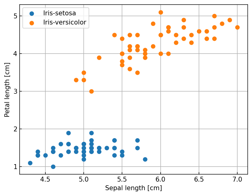
ax = plt.figure().gca()
for label in labels:
    mask = y == label
    ax.scatter(X[mask, 0], X[mask, 1], label=label)

ax.set(xlabel='Sepal length [cm]', ylabel='Petal length [cm]')
ax.legend();
Fitting a dataset with X: (100, 2) and y: (100,)
There are 50 examples of Iris-versicolor
Step 1 - Define and fit Adaline class
class Adaline:
    """ Parameters:
        -----------
        alpha : float - Learning rate between 0 and 1
        num_epochs : int - Iterations over the trainind ata
        random_seed : int - Random seed

        Attributes:
        -----------
        w_ : 1d array of weights
        b_ : bias term
    """
    def __init__(self, alpha=0.01, num_epochs=100, random_seed=42):
        self.alpha = alpha
        self.num_epochs = num_epochs
        self.random_seed = random_seed

    def fit(self, X, y):
        """ X : ndarray with shape [n_examples, n_features]
            y : ndarray with shape [n_examples,]
        """
        np.random.seed(self.random_seed)
        self.w_ = np.random.normal(loc=0., scale=0.1, size=X.shape[1])
        self.b_ = np.float32(0.)

        self.loss = []

        # iterate over epochs
        for _ in range(self.num_epochs):
            # Vectorize loss computation over the entire dataset
            diff = y - self.pre_threshold(X)
            self.w_ += 2. * self.alpha * diff.dot(X) / X.shape[0]
            self.b_ += 2. * self.alpha * diff.mean()

            loss = np.power(diff, 2).mean()

            self.loss.append(loss)

        return self

    def pre_threshold(self, X):
        return np.dot(X, self.w_) + self.b_

    def predict(self, X):
        z = self.pre_threshold(X)
        return np.where(z >= 0.5, 1, 0)
model = Adaline()
model.fit(X, y_enc)<__main__.Adaline at 0x7f79c3b2bed0>ax = plt.figure().gca()
ax.plot(model.loss)
ax.set(xlabel='Epochs', ylabel='MSE Loss');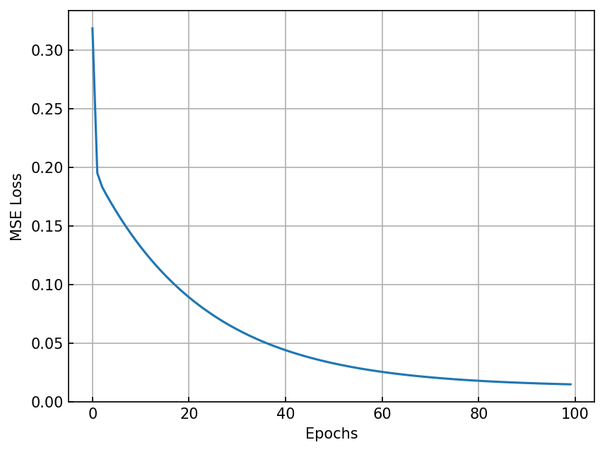
Step 2: Plot decision boundary
from matplotlib.colors import ListedColormap
def plot_decision_boundary(ax, X, y, model, d=0.05, colors=['red', 'blue']):
    x1, x2 = np.meshgrid(
        np.arange(X[:, 0].min() - 10*d, X[:, 0].max() + 10*d, d),
        np.arange(X[:, 1].min() - 10*d, X[:, 1].max() + 10*d, d),
    )
    y_grid = model.predict(np.stack([x1.ravel(), x2.ravel()]).T) # [N, 2]
    y_grid = y_grid.reshape(x1.shape)

    cmap = ListedColormap(colors)
    im = ax.pcolormesh(x1, x2, y_grid, cmap=cmap, alpha=0.5)

    for ii, label in enumerate(np.unique(y)):
        mask = y == label
        ax.scatter(X[mask, 0], X[mask, 1], color=colors[int(label)])

ax = plt.figure().gca()
plot_decision_boundary(ax, X, y_enc, model)
ax.set(xlabel='Sepal length [cm]', ylabel='Petal length [cm]');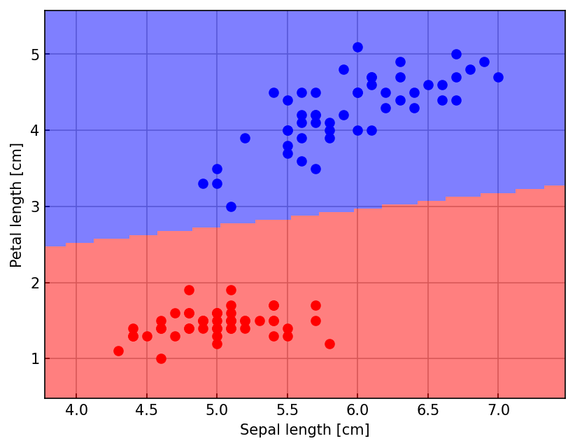
Step 3 : Train the Adaline model at different learning rates
ax = plt.figure().gca()

for alpha in [0.1, 0.01, 0.001]:
    model_alpha = Adaline(alpha=alpha, num_epochs=100)
    model_alpha.fit(X, y_enc)
    ax.plot(model_alpha.loss, label=f'$\\alpha$ = {alpha:g}')
ax.set(xlabel='Epochs', ylabel='MSE Loss', yscale='log', ylim=[1e-2, 1e3]);
ax.legend();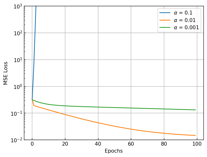
Step 4: See the benefit of feature scaling
X_std = (X - np.mean(X, axis=0)) / np.std(X, axis=0)
model_scaled = Adaline(alpha=0.1, num_epochs=100).fit(X_std, y_enc)

ax = plt.figure().gca()
ax.plot(model_scaled.loss, label=f'$\\alpha$ = {model.alpha:g} with feature scaling')
ax.set(xlabel='Epochs', ylabel='MSE Loss', yscale='log');
ax.legend()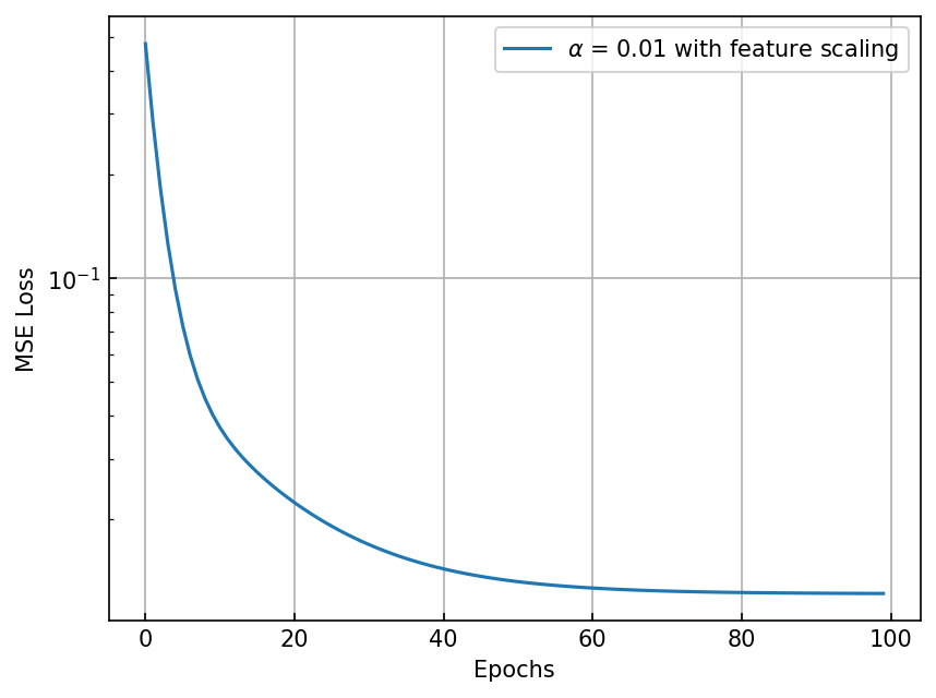
Step 5: Plot the decision boundary in scaled coordinates
from matplotlib.colors import ListedColormap
ax = plt.figure().gca()
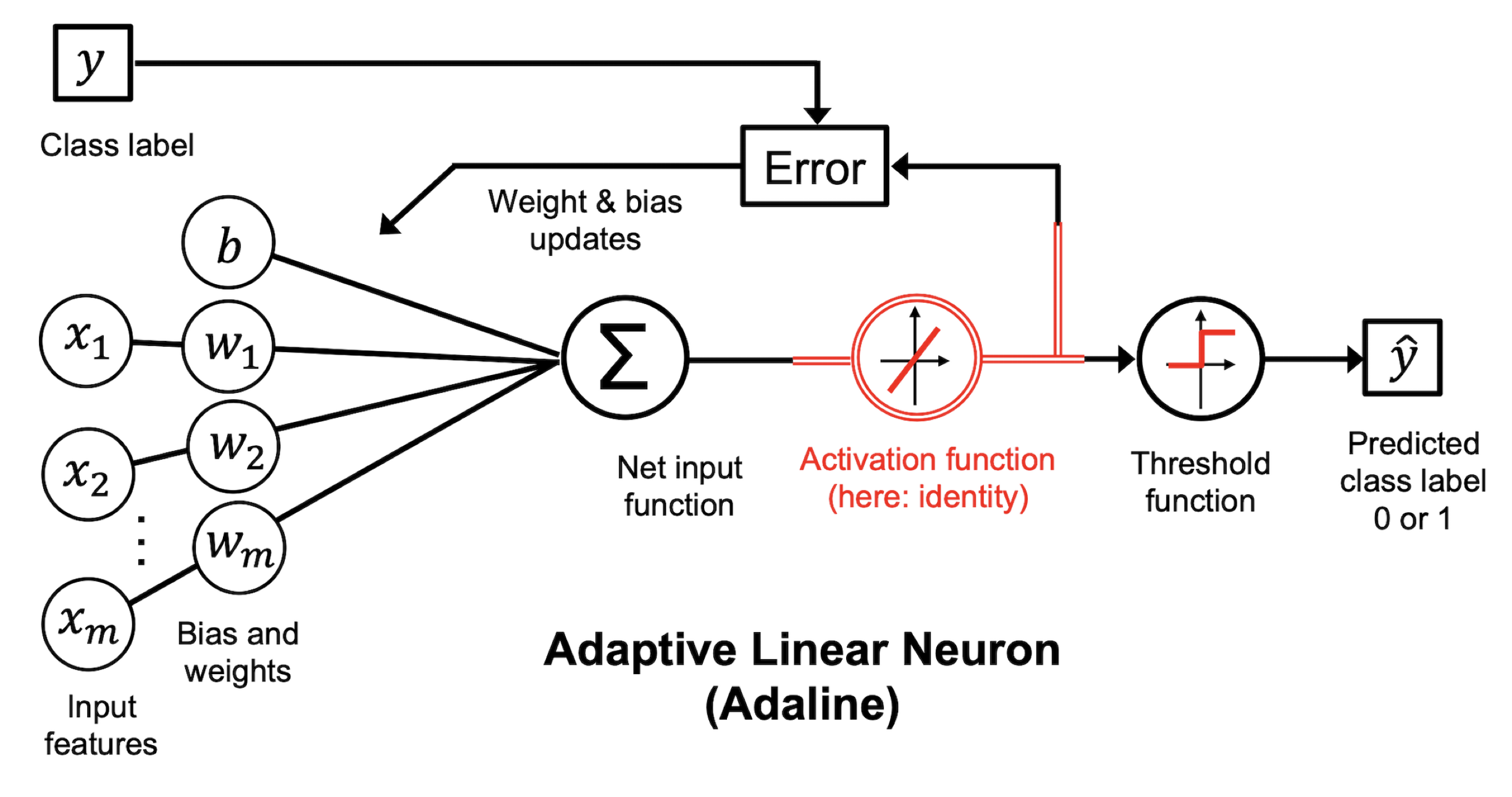
plot_decision_boundary(ax, X_std, y_enc, model_scaled)