Deep Neural Networks (from scratch)
%matplotlib inline
import numpy as np
import matplotlib.pyplot as plt
import seaborn as sns
import pandas as pd
plt.rcParams['xtick.direction'] = 'in'
plt.rcParams['ytick.direction'] = 'in'
Dataset: MNIST handwritten digits
This is a publicly-available handwritten digit dataset link. It’s also available in nearly every ML library
from sklearn.datasets import fetch_openml

X, y = fetch_openml('mnist_784', version=1, return_X_y=True)
X = X.values
y = y.astype(int).values

print('Inputs have size', X.shape)
print('Targets have size', y.shape)
Inputs have size (70000, 784)
Targets have size (70000,)
Let’s visualize one example from each input class
fig, ax = plt.subplots(2, 5, sharex=True, sharey=True)
ax = ax.flatten()
for ii in range(10):
    example_img = X[y == ii][0].reshape([28, 28])
    ax[ii].imshow(example_img, cmap='Greys')
    ax[ii].set(xticks=[], yticks=[])
plt.tight_layout()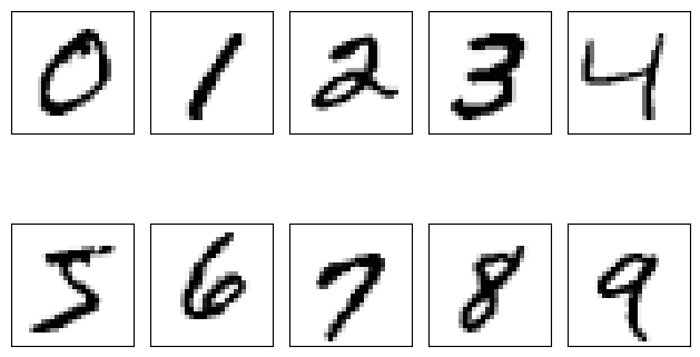
To visualize the distribution of possible inputs, let’s use PCA
from sklearn.decomposition import PCA
pca = PCA(n_components=2, whiten=True)

X_pca = pca.fit_transform(X)

ax = plt.figure().gca()
for ii in range(10):
    mask = y == ii
    ax.scatter(X_pca[mask, 0], X_pca[mask, 1], s=1, label=ii)
ax.set(xlabel='Principal Component 1', ylabel='Principal Component 2')
ax.legend()
plt.tight_layout()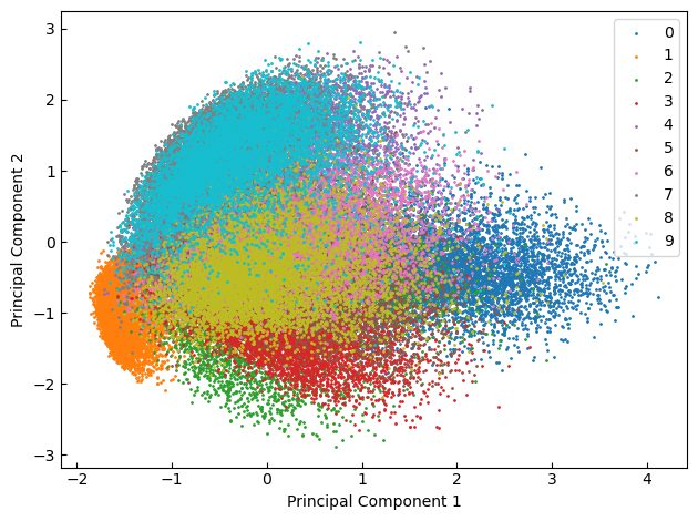
To prepare for our deep learning expedition, let’s get a training, validation, and test set
from sklearn.model_selection import train_test_split
from sklearn.preprocessing import OneHotEncoder, MinMaxScaler

def normalize(X):
    """ X is a uint8 that takes values from 0 to 255.
        Convert it to a float between -1 and 1
    """
    return 2. * X / 255. - 1.

label_encoder = OneHotEncoder(sparse_output=False) # Sparse output makes downstream work a bit annoying
y_enc = label_encoder.fit_transform(y[:, None])

X_train, X_test, y_train, y_test = train_test_split(normalize(X), y_enc, test_size=0.2, random_state=42)
X_train, X_val, y_train, y_val = train_test_split(X_train, y_train, test_size=0.2, random_state=42)

print(f"The training set has size {X_train.shape}, {y_train.shape}")
print(f"The validation set has size {X_val.shape}, {y_val.shape}")
print(f"The testing set has size {X_test.shape}, {y_test.shape}")
The training set has size (44800, 784), (44800, 10)
The validation set has size (11200, 784), (11200, 10)
The testing set has size (14000, 784), (14000, 10)
Finally, let’s establish a baseline. We are going to use mean-squared error loss here
PS1 will cover cross entropy loss.
def mse_loss(y_true, y_pred):
    return np.mean(
        np.power(y_true - y_pred, 2).sum(axis=1)
    )

def accuracy(y_true, y_pred):
    y_label = np.argmax(y_true, axis=1)
    pred_label = np.argmax(y_pred, axis=1)
    return np.mean(y_label == pred_label)
Logistic regression is as good a place as any to start. But this time we’ll use the sklearn implementation rather than our own. This uses a 2nd order L-BFGS solver which should in principle do a bit better than gradient descent.
from sklearn.linear_model import LogisticRegression

# Initialize and fit the model
lr_model = LogisticRegression(max_iter=10)
lr_model.fit(X_train, label_encoder.inverse_transform(y_train)[:, 0])

# Measure the training set performance
y_train_pred = lr_model.predict_proba(X_train)
train_mse = mse_loss(y_train, y_train_pred)
train_acc = accuracy(y_train, y_train_pred)
print(f"Train MSE = {train_mse:.3f}\tTrain Accuracy = {train_acc:.3f}")

# Measure the testing set performance
y_test_pred = lr_model.predict_proba(X_test)
test_mse = mse_loss(y_test, y_test_pred)
test_acc = accuracy(y_test, y_test_pred)
print(f"Test MSE = {test_mse:.3f}\tTest Accuracy = {test_acc:.3f}")
/opt/conda/lib/python3.11/site-packages/sklearn/linear_model/_logistic.py:469: ConvergenceWarning: lbfgs failed to converge (status=1):
STOP: TOTAL NO. of ITERATIONS REACHED LIMIT.
Increase the number of iterations (max_iter) or scale the data as shown in:
https://scikit-learn.org/stable/modules/preprocessing.html
Please also refer to the documentation for alternative solver options:
https://scikit-learn.org/stable/modules/linear_model.html#logistic-regression
n_iter_i = _check_optimize_result(
Train MSE = 0.226	Train Accuracy = 0.844
Test MSE = 0.223	Test Accuracy = 0.847
import numpy as np

class MLP_2Layer:
    def __init__(self,
                 num_inputs,
                 num_hidden,
                 num_outputs,
                 random_seed=42):
        self.num_inputs = num_inputs
        self.num_hidden = num_hidden
        self.num_outputs = num_outputs
        self.random_seed = random_seed
        self._initialize_weights()

    def _initialize_weights(self):
        np.random.seed(self.random_seed)

        # Initialize hidden layer weights and biases
        self.w_hidden = np.random.normal(loc=0, scale=0.1,
                                         size=(self.num_inputs, self.num_hidden))
        self.b_hidden = np.zeros(self.num_hidden)

        # Initialize output layer weights and biases
        self.w_output = np.random.normal(loc=0, scale=0.1,
                                         size=(self.num_hidden, self.num_outputs))
        self.b_output = np.zeros(self.num_outputs)

    def forward(self, x):
        """ Feed input data x through each network layer
            Return a final network output, as well as the intermediate
            values at each layer
        """
        # Apply hidden layer functions
        z_hidden = np.dot(x, self.w_hidden) + self.b_hidden
        a_hidden = 1. / (1 + np.exp(-np.clip(z_hidden, -250, 250)))

        # Apply output layer function
        z_output = np.dot(a_hidden, self.w_output) + self.b_output
        a_output = 1. / (1 + np.exp(-np.clip(z_output, -250, 250)))

        return a_output, (
            a_output,
            z_output,
            a_hidden,
            z_hidden,
        )

    def backward(self, x, y_true, a_output, z_output, a_hidden, z_hidden):
        """ Compute gradients with respect to each model parameter """
        # Sanity check on input shapes
        B, I = x.shape # [B, I]
        _, O = y_true.shape # [B, O]
        assert y_true.shape[0] == B

        # Compute gradients w.r.t. output layer preactivation
        # Should be same size as z_output: [B, O]
        d_loss__d_a_output = 2. * (a_output - y_true) / B # [B, O]
        d_a_output__d_z_output = a_output * (1 - a_output) # [B, O]
        d_loss__d_z_output = d_loss__d_a_output * d_a_output__d_z_output # [B, O]

        # Compute gradients w.r.t. output layer weights
        # Should be same size as w_output: [H, O]
        d_z_output__d_w_output = a_hidden # [B, H]
        d_loss__d_w_output = np.matmul(d_z_output__d_w_output.T, d_loss__d_z_output)
        # [B, H].T x [B, O] = [H, B] x [B, O] -> [H, O]

        # Compute gradients w.r.t. output layer biases
        # Should be same size as b_output: [O,]
        d_z_output__d_b_output = 1.
        d_loss__d_b_output = np.sum(d_loss__d_z_output, axis=0) * d_z_output__d_b_output

        # Compute gradients w.r.t. hidden layer preactivation
        # Should be same size as z_hidden: [B, H]
        d_z_output__d_a_hidden = self.w_output # [H, O]
        d_loss__d_a_hidden = np.matmul(d_loss__d_z_output, d_z_output__d_a_hidden.T)
        # [B, O] x [H, O].T = [B, O] x [O, H] -> [B, H]

        d_a_hidden__d_z_hidden = a_hidden * (1. - a_hidden)
        d_loss__d_z_hidden = d_loss__d_a_hidden * d_a_hidden__d_z_hidden

        # Compute gradients w.r.t. hidden layer weights
        # Should be same size as w_hidden: [I, H]
        d_z_hidden__d_w_hidden = x # [B, I]
        d_loss__d_w_hidden = np.matmul(d_z_hidden__d_w_hidden.T, d_loss__d_z_hidden)
        # [B, I].T x [B, H] = [I, B] x [B, H] -> [I, H]

        # Compute gradients w.r.t. hidden layer biases
        # Should be same size as b_hidden: [H,]
        d_z_hidden__d_b_hidden = 1.
        d_loss__d_b_hidden = np.sum(d_loss__d_z_hidden, axis=0) * d_z_hidden__d_b_hidden

        # We're done. Return all the gradients w.r.t. weights and biases
        return d_loss__d_w_output, \
               d_loss__d_b_output, \
               d_loss__d_w_hidden, \
               d_loss__d_b_hidden

    def weight_update(self, d_loss__d_w_output, d_loss__d_b_output, d_loss__d_w_hidden, d_loss__d_b_hidden, lr=0.3):
        """ Update weights and biases via gradient descent
        """
        self.w_output -= lr * d_loss__d_w_output
        self.b_output -= lr * d_loss__d_b_output
        self.w_hidden -= lr * d_loss__d_w_hidden
        self.b_hidden -= lr * d_loss__d_b_hidden
model = MLP_2Layer(num_inputs=X_train.shape[1],
num_hidden=64,
num_outputs=y_train.shape[1])y_pred, _ = model.forward(X_val)
mse = mse_loss(y_val, y_pred)
acc = accuracy(y_val, y_pred)
print(f'Initial Val MSE: {mse:.3f}, Val Accuracy: {acc:.3f}')Initial Val MSE: 2.610, Val Accuracy: 0.125
Training the model
def batch_loader(X, y, batch_size=32):
    """ Iterator that produces batches of a particular size """
    indices = np.arange(X.shape[0])
    np.random.shuffle(indices)

    for start in range(0, indices.shape[0] - batch_size + 1, batch_size):
        batch_idx = indices[start:start+batch_size]
        yield X[batch_idx], y[batch_idx]

loader = batch_loader(X_train, y_train, batch_size=32)
Xb, yb = next(loader)
print(Xb.shape, yb.shape)
(32, 784) (32, 10)
from tqdm.auto import tqdm, trange

def train(model,
          X_train,
          y_train,
          X_val,
          y_val,
          num_epochs=10,
          lr=0.3,
          lr_decay=1.,
          batch_size=128):
    """ Standalone function to execute the mini-batch SGD training loop

        Parameters:
        -----------
        X_train, y_train: Training dataset
        X_val, y_val: Validation dataset
        num_epochs: number of passes through the dataset, use 10 for consistent comparison with LR above
        batch_size: number of samples in each minibatch
        lr: learning rate for gradient updates
        lr_decay: decreases the learning rate, may aid SGD convergence
    """
    train_mse, train_acc = [], []
    val_mse, val_acc = [], []

    pbar_epoch = trange(num_epochs)
    for ii in pbar_epoch:
        loader = batch_loader(X_train, y_train, batch_size=batch_size)
        for Xb, yb in tqdm(loader, position=1, leave=False, total=X_train.shape[0] // batch_size):
            # Make the prediction
            y_pred, layer_values = model.forward(Xb)
            # Compute the gradients
            gradients = model.backward(Xb, yb, *layer_values)

            # Update the weights
            model.weight_update(*gradients, lr=lr)

        # Compute loss, accuracy on training set
        y_train_pred, _ = model.forward(X_train)
        train_mse.append(mse_loss(y_train, y_train_pred))
        train_acc.append(accuracy(y_train, y_train_pred))

        # Compute loss, accuracy on validation set
        y_val_pred, _ = model.forward(X_val)
        val_mse.append(mse_loss(y_val, y_val_pred))
        val_acc.append(accuracy(y_val, y_val_pred))

        pbar_epoch.set_postfix(
            epoch=f"{ii+1:03d} / {num_epochs:03d}",
            train_mse=f"{train_mse[-1]:.3f}",
            train_acc=f"{train_acc[-1]:.3f}",
            val_mse=f"{val_mse[-1]:.3f}",
            val_acc=f"{val_acc[-1]:.3f}")

        lr *= lr_decay # This aids SGD convergence by lowering the step size over time

    return train_mse, train_acc, val_mse, val_acc
model = MLP_2Layer(num_inputs=X_train.shape[1],
num_hidden=64,
num_outputs=y_train.shape[1])
train_mse, train_acc, val_mse, val_acc = train(model, X_train, y_train, X_val, y_val)Plot training curves
fig, ax = plt.subplots(1, 2, sharex=True, figsize=(5, 2.5))

# Plot training and validation MSE on axis 0
ax[0].plot(train_mse, color='black')
ax[0].plot(val_mse, color='red')
ax[0].set(xlabel='Epoch', ylabel='MSE Loss')

# Plot training and validation accuracy on axis 1
ax[1].plot(train_acc, color='black', label='Train')
ax[1].plot(val_acc, color='red', label='Validation')
ax[1].set(xlabel='Epoch', ylabel='Accuracy')

fig.legend(*ax[1].get_legend_handles_labels(),
           loc='center left', bbox_to_anchor=[1, 0.5], framealpha=0)

plt.tight_layout()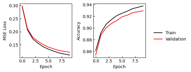
Evaluate test accuracy
# Make predictions on the test set here
y_test_pred, _ = model.forward(X_test)
test_mse = mse_loss(y_test, y_test_pred)
test_acc = accuracy(y_test, y_test_pred)
print(f"Test MSE = {test_mse:.3f}\tTest Accuracy = {test_acc:.3f}")
Test MSE = 0.117 Test Accuracy = 0.932
Examine failed cases
wrong = np.where(np.argmax(y_test_pred, axis=1) != np.argmax(y_test, axis=1))[0]

fig, ax = plt.subplots(2, 5, figsize=(10, 4), sharex=True, sharey=True)
ax = ax.flatten()

for ii in range(10):
    img = X_test[wrong[ii], :].reshape([28, 28])
    true_label = np.argmax(y_test[wrong[ii]])
    pred_label = np.argmax(y_test_pred[wrong[ii]])

    ax[ii].imshow(img, cmap='Greys')
    ax[ii].set(xticks=[], yticks=[], title=f"True: {true_label}\nPredicted: {pred_label}")

plt.tight_layout()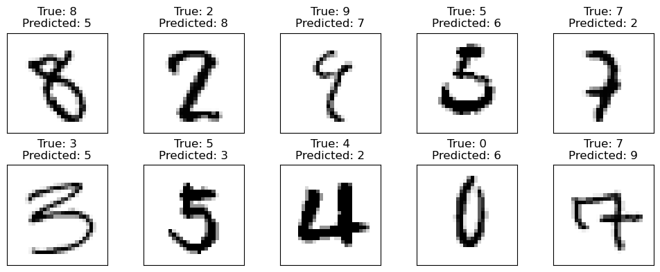
What does the model learn?
Each hidden layer neuron is sensitive to a particular pixel configuration. We can visualize this to get an understanding for the input representations that the model produces.
model.w_hidden.shape(784, 64)fig, axes = plt.subplots(8, 8, figsize=(10, 10), dpi=150)
for weights, ax in zip(model.w_hidden.T, axes.ravel()):
w_img = weights.reshape([28,28])
ax.imshow(w_img, cmap='bwr', vmin=-1, vmax=1)
ax.set(xticks=[], yticks=[])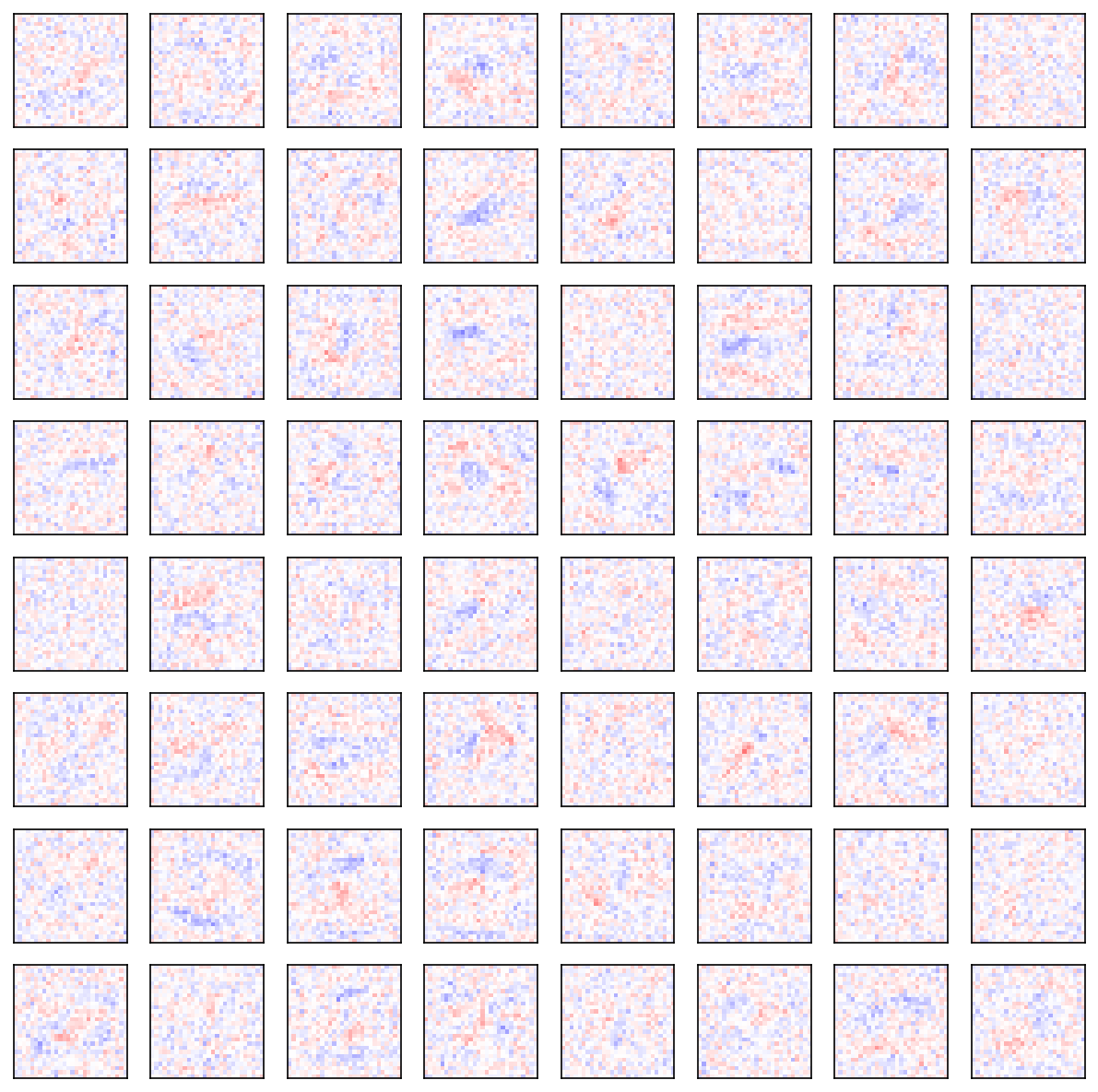
Variations
To aid in the examples below, it’s useful to have these helper functions
Helper functions
import numpy as np

def preactivation(x, w, b):
    """ Applies weights and biases
    """
    return np.dot(x, w) + b

def grad_preactivation(x, w, b, z):
    """ Accepts inputs x, w, b, output z
        Returns gradient of output w.r.t. each input
    """
    dz_dx = w
    dz_dw = x
    dz_db = 1.
    return dz_dx, dz_dw, dz_db

def sigmoid(z):
    """ Squashing activation function
    """
    return 1. / (1. + np.exp(-np.clip(z, -250, 250)))

def grad_sigmoid(z, a):
    """ Accepts input z, output a
        Returns gradient of output w.r.t. input
    """
    return a * (1. - a)

def relu(z):
    """ Thresholded ramp activation function
    """
    return np.maximum(0, z)

def grad_relu(z, a):
    """ Accepts input z, output a
        Returns gradient of output w.r.t. input
    """
    return np.where(z >= 0, 1., 0.)

def mse_loss(y_true, y_pred):
    """ Mean squared error
    """
    return np.mean(
        np.power(y_true - y_pred, 2).sum(axis=1)
    )

def grad_mse_loss(y_true, y_pred):
    """ Returns gradient of MSE loss w.r.t. model prediction y_pred
    """
    return 2. / y_true.shape[0] * (y_pred - y_true)
ReLU MLP
Consider an MLP whose hidden layer uses the ReLU function instead of sigmoid. ReLU is defined as
[Question:] What is its derivative?
With this our network is now defined as
import numpy as np

class MLP_2Layer_ReLU:
    def __init__(self,
                 num_inputs,
                 num_hidden,
                 num_outputs,
                 random_seed=42):
        self.num_inputs = num_inputs
        self.num_hidden = num_hidden
        self.num_outputs = num_outputs
        self.random_seed = random_seed
        self._initialize_weights()

    def _initialize_weights(self):
        np.random.seed(self.random_seed)

        # Initialize hidden layer weights and biases
        self.w_hidden = np.random.normal(loc=0, scale=0.1,
                                         size=(self.num_inputs, self.num_hidden))
        self.b_hidden = np.zeros(self.num_hidden)

        # Initialize output layer weights and biases
        self.w_output = np.random.normal(loc=0, scale=0.1,
                                         size=(self.num_hidden, self.num_outputs))
        self.b_output = np.zeros(self.num_outputs)

    def forward(self, x):
        """ Feed input data x through each network layer
            Return a final network output, as well as the intermediate
            values at each layer
        """
        # Apply hidden layer functions
        z_hidden = preactivation(x, self.w_hidden, self.b_hidden)
        a_hidden = relu(z_hidden)

        # Apply output layer function
        z_output = preactivation(a_hidden, self.w_output, self.b_output)
        a_output = sigmoid(z_output)

        return a_output, (
            a_output,
            z_output,
            a_hidden,
            z_hidden,
        )

    def backward(self, x, y_true, a_output, z_output, a_hidden, z_hidden):
        """ Compute gradients with respect to each model parameter """
        # Sanity check on input shapes
        B, I = x.shape # [B, I]
        _, O = y_true.shape # [B, O]
        assert y_true.shape[0] == B

        # Compute gradients w.r.t. output layer preactivation
        # Should be same size as z_output: [B, O]
        d_loss__d_a_output = grad_mse_loss(y_true, a_output) #[B, O]
        d_a_output__d_z_output = grad_sigmoid(z_output, a_output) #[B, O]
        d_loss__d_z_output = d_loss__d_a_output * d_a_output__d_z_output #[B, O]

        # Compute gradients w.r.t. output layer weights
        # Should be same size as w_output: [H, O]
        d_z_output__d_w_output = a_hidden #[B, H]
        d_loss__d_w_output = np.einsum('Bo,Bh->ho', d_loss__d_z_output, d_z_output__d_w_output)

        # Compute gradients w.r.t. output layer biases
        # Should be same size as b_output: [O,]
        d_z_output__d_b_output = 1.
        d_loss__d_b_output = np.einsum('Bo,->o', d_loss__d_z_output, d_z_output__d_b_output)

        # Compute gradients w.r.t. hidden layer preactivation
        # Should be same size as z_hidden: [B, H]
        d_z_output__d_a_hidden = self.w_output #[H, O]
        d_loss__d_a_hidden = np.einsum('Bo,ho->Bh', d_loss__d_z_output, d_z_output__d_a_hidden)

        d_a_hidden__d_z_hidden = grad_relu(z_hidden, a_hidden) #[B, H]
        d_loss__d_z_hidden = d_loss__d_a_hidden * d_a_hidden__d_z_hidden #[B, H]

        # Compute gradients w.r.t. hidden layer weights
        # Should be same size as w_hidden: [I, H]
        d_z_hidden__d_w_hidden = x #[B, I]
        d_loss__d_w_hidden = np.einsum('Bh,Bi->ih', d_loss__d_z_hidden, d_z_hidden__d_w_hidden)

        # Compute gradients w.r.t. hidden layer biases
        # Should be same size as b_hidden: [H,]
        d_z_hidden__d_b_hidden = 1.
        d_loss__d_b_hidden = np.einsum('Bh,->h', d_loss__d_z_hidden, d_z_hidden__d_b_hidden)

        # We're done. Return all the gradients w.r.t. weights and biases
        return d_loss__d_w_output, \
               d_loss__d_b_output, \
               d_loss__d_w_hidden, \
               d_loss__d_b_hidden

    def weight_update(self, d_loss__d_w_output, d_loss__d_b_output, d_loss__d_w_hidden, d_loss__d_b_hidden, lr=0.3):
        """ Update weights and biases via gradient descent
        """
        self.w_output -= lr * d_loss__d_w_output
        self.b_output -= lr * d_loss__d_b_output
        self.w_hidden -= lr * d_loss__d_w_hidden
        self.b_hidden -= lr * d_loss__d_b_hidden
model = MLP_2Layer_ReLU(num_inputs=X_train.shape[1],
num_hidden=64,
num_outputs=y_train.shape[1])
train_mse, train_acc, val_mse, val_acc = train(model, X_train, y_train, X_val, y_val, lr=0.1)# Make predictions on the test set here
y_test_pred, _ = model.forward(X_test)
test_mse = mse_loss(y_test, y_test_pred)
test_acc = accuracy(y_test, y_test_pred)
print(f"Test MSE = {test_mse:.3f}\tTest Accuracy = {test_acc:.3f}")Test MSE = 0.108 Test Accuracy = 0.938
3-layer MLP
class MLP_3Layer:
    def __init__(self,
                 num_inputs,
                 num_hidden,
                 num_outputs,
                 random_seed=42):
        self.num_inputs = num_inputs
        self.num_hidden = num_hidden
        self.num_outputs = num_outputs
        self.random_seed = random_seed

        # Left to child classes
        self._initialize_weights()

    def _initialize_weights(self):
        np.random.seed(self.random_seed)

        # Initialize hidden layer weights and biases
        self.w_h1 = np.random.normal(loc=0, scale=0.1,
                                     size=(self.num_inputs, self.num_hidden))
        self.b_h1 = np.zeros(self.num_hidden)

        self.w_h2 = np.random.normal(loc=0, scale=0.1,
                                     size=(self.num_hidden, self.num_hidden))
        self.b_h2 = np.zeros(self.num_hidden)

        # Initialize output layer weights and biases
        self.w_o = np.random.normal(loc=0, scale=0.1,
                                    size=(self.num_hidden, self.num_outputs))
        self.b_o = np.zeros(self.num_outputs)

    def forward(self, x):
        """ Feed input data x through each network layer
            Return a final network output, as well as the intermediate
            values at each layer
        """
        # Apply hidden layer functions
        z_h1 = preactivation(x, self.w_h1, self.b_h1)
        a_h1 = relu(z_h1)

        z_h2 = preactivation(a_h1, self.w_h2, self.b_h2)
        a_h2 = relu(z_h2)

        # Apply output layer function
        z_o = preactivation(a_h2, self.w_o, self.b_o)
        a_o = sigmoid(z_o)

        return a_o, (
            a_o,
            z_o,
            a_h2,
            z_h2,
            a_h1,
            z_h1
        )

    def backward(self, x, y_true, a_o, z_o, a_h2, z_h2, a_h1, z_h1):
        """ Compute gradients with respect to each model parameter """
        B, I = x.shape # [B, I]
        _, O = y_true.shape # [B, O]
        assert y_true.shape[0] == B

        # Start by computing gradients w.r.t. model prediction
        d_loss__d_a_o = grad_mse_loss(y_true, a_o) #[B, O]

        # Output layer
        d_a_o__d_z_o = grad_sigmoid(z_o, a_o)
        d_loss__d_z_o = d_loss__d_a_o * d_a_o__d_z_o

        d_z_o__d_a_h2, d_z_o__d_w_o, d_z_o__d_b_o = \
            grad_preactivation(a_h2, self.w_o, self.b_o, z_o)
        d_loss__d_w_o = np.einsum('Bo,Bh->ho', d_loss__d_z_o, d_z_o__d_w_o)
        d_loss__d_b_o = np.einsum('Bo,->o', d_loss__d_z_o, d_z_o__d_b_o)
        d_loss__d_a_h2 = np.einsum('Bo,ho->Bh', d_loss__d_z_o, d_z_o__d_a_h2)

        # 2nd hidden layer
        d_a_h2__d_z_h2 = grad_relu(z_h2, a_h2)
        d_loss__d_z_h2 = d_loss__d_a_h2 * d_a_h2__d_z_h2

        d_z_h2__d_a_h1, d_z_h2__d_w_h2, d_z_h2__d_b_h2 = \
            grad_preactivation(a_h1, self.w_h2, self.b_h2, z_h2)
        d_loss__d_w_h2 = np.einsum('Bo,Bh->ho', d_loss__d_z_h2, d_z_h2__d_w_h2)
        d_loss__d_b_h2 = np.einsum('Bo,->o', d_loss__d_z_h2, d_z_h2__d_b_h2)
        d_loss__d_a_h1 = np.einsum('Bo,ho->Bh', d_loss__d_z_h2, d_z_h2__d_a_h1)

        # 1st hidden layer
        d_a_h1__d_z_h1 = grad_relu(z_h1, a_h1)
        d_loss__d_z_h1 = d_loss__d_a_h1 * d_a_h1__d_z_h1

        d_z_h1__d_x, d_z_h1__d_w_h1, d_z_h1__d_b_h1 = \
            grad_preactivation(x, self.w_h1, self.b_h1, z_h1)
        d_loss__d_w_h1 = np.einsum('Bo,Bh->ho', d_loss__d_z_h1, d_z_h1__d_w_h1)
        d_loss__d_b_h1 = np.einsum('Bo,->o', d_loss__d_z_h1, d_z_h1__d_b_h1)

        return d_loss__d_w_o, d_loss__d_b_o, \
               d_loss__d_w_h2, d_loss__d_b_h2, \
               d_loss__d_w_h1, d_loss__d_b_h1

    def weight_update(self, grad_w_o, grad_b_o, grad_w_h2, grad_b_h2, grad_w_h1, grad_b_h1, lr=0.3):
        """ Update weights and biases via gradient descent
        """
        self.w_o -= lr * grad_w_o
        self.b_o -= lr * grad_b_o
        self.w_h2 -= lr * grad_w_h2
        self.b_h2 -= lr * grad_b_h2
        self.w_h1 -= lr * grad_w_h1
        self.b_h1 -= lr * grad_b_h1
model = MLP_3Layer(num_inputs=X_train.shape[1],
                   num_hidden=64,
                   num_outputs=y_train.shape[1])
train_mse, train_acc, val_mse, val_acc = train(model, X_train, y_train, X_val, y_val)# Make predictions on the test set here
y_test_pred, _ = model.forward(X_test)
test_mse = mse_loss(y_test, y_test_pred)
test_acc = accuracy(y_test, y_test_pred)
print(f"Test MSE = {test_mse:.3f}\tTest Accuracy = {test_acc:.3f}")Test MSE = 0.063 Test Accuracy = 0.961
N-layer MLP
It would be nice to have a framework to build arbitrarily deep multi-layer perceptrons without having to type so much, right? There is a compositional structure to these, so we should be able to loop some of the computation. For example, each layer generally computes
class MLP_Layer:
    """ To reduce redundancy, we're going to implement a standalone MLP layer.
        This will implement:
            1. forward function that computes a preactivation and an activation
            2. backward function that computes gradients w.r.t. each parameter
            3. weight_update function that updates weight values using a particular learning rate
    """
    def __init__(self,
                 num_inputs,
                 num_outputs,
                 activation,
                 grad_activation):

        self.num_inputs = num_inputs
        self.num_outputs = num_outputs
        self.activation = activation
        self.grad_activation = grad_activation

        self.w_ =
        self.b_ =

    def preactivation(self, x):
        z =
        return z

    def grad_preactivation(self, x, z):
        dz_dx =
        dz_dw =
        dz_db =
        return dz_dx, dz_dw, dz_db

    def forward(self, x):
        z = self.preactivation(x)
        a = self.activation(z)
        return a, z

    def backward(self, a, z, x, d_loss__d_a):
        """ d_loss__d_a is the gradient w.r.t. the output of this layer
            It is computed upstream and passed here via backpropagation.
        """
        # Compute gradient w.r.t. preactivation
        d_a__d_z = self.grad_activation(z, a)
        d_loss__d_z =

        # Compute gradient w.r.t. input, weight, bias
        d_z__d_x, d_z__d_w, d_z__d_b = self.grad_preactivation(x, z)

        d_loss__d_x =
        d_loss__d_w =
        d_loss__d_b =

        return d_loss__d_x, d_loss__d_w, d_loss__d_b

    def weight_update(self, grad_w, grad_b, lr):
        self.w_ -= lr * grad_w
        self.b_ -= lr * grad_b
class MLP_NLayer:
""" More general N-layer architecture
"""
def __init__(self,
num_inputs,
num_hidden,
num_hidden_layers,
num_outputs,
random_seed=42):
self.num_inputs = num_inputs
self.num_hidden = num_hidden
self.num_hidden_layers = num_hidden_layers
self.num_outputs = num_outputs
self.random_seed = random_seed
self._initialize_weights()
def _initialize_weights(self):
np.random.seed(self.random_seed)
self.layers = []
# Initialize hidden layers
for ii in range(self.num_hidden_layers):
# Initialize output layer
def forward(self, x):
""" Feed input data x through each network layer
Return a final network output, as well as the intermediate
values at each layer
"""
# Apply hidden layer functions in order
# Store preactivations and activations in a list called layer_values
layer_values = [x,]
for layer in self.layers:
return x, layer_values
def backward(self, x, y_true, *layer_values):
""" Compute gradients with respect to each model parameter """
B, I = x.shape # [B, I]
_, O = y_true.shape # [B, O]
assert y_true.shape[0] == B
# Iterate through layers backward
layers = self.layers[::-1]
values = layer_values[::-1]
# Start by computing gradient of loss w.r.t. final layer output
d_loss__d_a =
# At each step, I need to pass the layer input, preactivation,
# and output to the gradient function
# layer_values is [x, z1, a1, z2, a2, ..., ,zo, ao]
outputs =
preacts =
inputs =
gradients = []
for layer, x, z, a in zip(layers, inputs, preacts, outputs):
# Do the computation in each layer
# We're done. Return all the gradients w.r.t. weights and biases
# Reverse them to be sure that they match the order of layers
return reversed(gradients)
def weight_update(self, *gradients, lr=0.3):
""" Update weights and biases via gradient descent
"""
for layer, (grad_w, grad_b) in zip(self.layers, gradients):
layer.weight_update(grad_w, grad_b, lr)