Image data and convolutional neural networks

%matplotlib inline
import numpy as np
import matplotlib.pyplot as plt
import seaborn as snss
import pandas as pd
plt.rcParams['xtick.direction'] = 'in'
plt.rcParams['ytick.direction'] = 'in'
plt.rcParams['axes.grid'] = True
plt.rcParams['axes.axisbelow'] = True
plt.rcParams['figure.dpi'] = 150

# Check available hardware
import torch
if torch.cuda.is_available():
    print(f'GPU is available, using GPU {torch.cuda.get_device_name(0)}')
    device = torch.device('cuda')
elif torch.mps.is_available():
    print(f'Apple Metal Performance Shaders framework is available, using {torch.device("mps")}')
    device = torch.device('mps')
else:
    print(f'Hardware acceleration not available, using CPU')
    device = torch.device('cpu')

GPU is available, using GPU NVIDIA A40

Original	Translated	Coarsened	Super-resolved

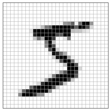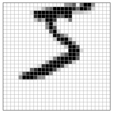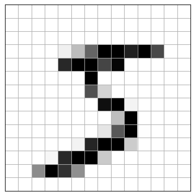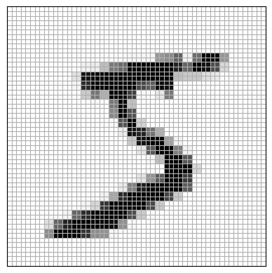Compared to structured tabular datasets like Iris, images pose some particular challenges. For example, the four images above all contain the same object. But they would be viewed very differently by an MLP.

Version	Vector
Original
Shifted
Coarsened
Super-resolved

If we trained a MLP only on centered MNIST images, the shifted image might cause a completely different set of activations in the hidden layer, leading to misclassification. And the coarsened/super-resolved images would have sizes that are incompatible with the hidden layer weight matrix.

Animal vision tends to overcome these problems, and CNNs are loosely inspired by experimental results on the visual cortex. These experiments revealed a hierarchical structure with simple and complex cells. The simple cells identify features such as edges within narrow visual regions, or receptive fields. The complex cells probe a larger region and their activation is less sensitive on the exact position of an object within their view.

Visual perception, therefore, roughly follows this process

\begin{align} \text{Retinal stimulation} \underbrace{\rightarrow}_{\text{Simple cells}} \text{Low-level features} \underbrace{\rightarrow}_{\text{Complex cells}} \text{High-level features} \underbrace{\rightarrow}_{\dots} \text{Recognition} \end{align}

Convolutional neural networks (CNN) aim to learn feature maps that incorporate several key aspects:

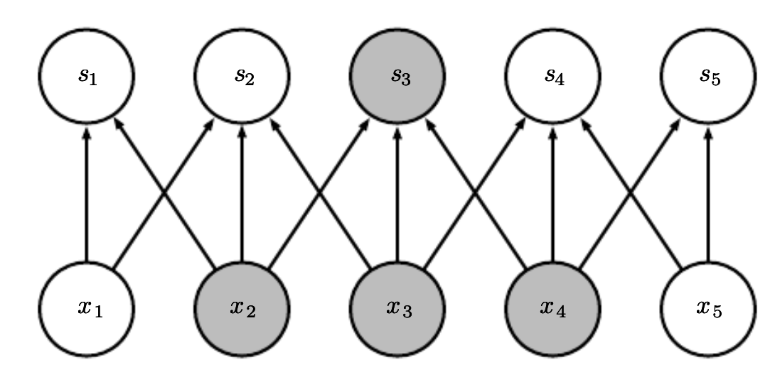
Sparse connectivity - like simple cells, each output of a CNN layer accesses only a small region of the input
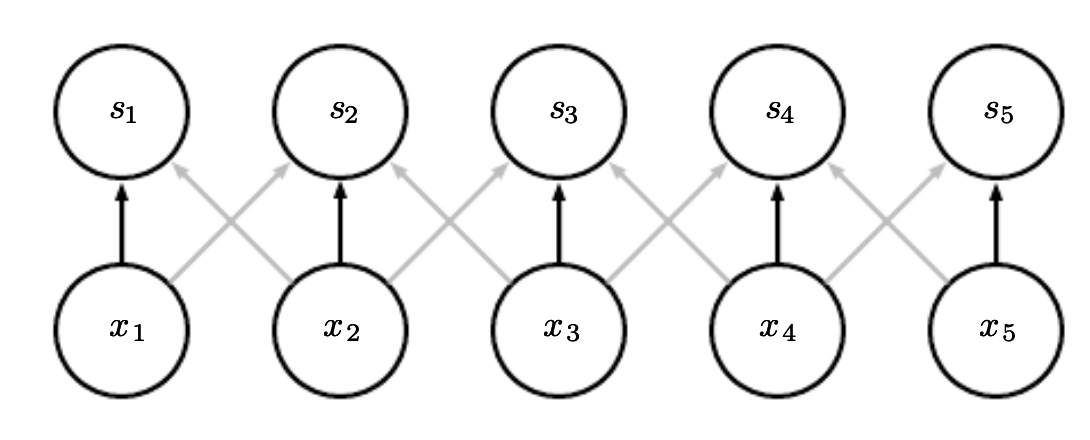
Weight sharing - like complex cells, CNNs produce outputs that are insensitive to position by applying the same weights at different places, and pooling the outputs

Combined, these properties give CNNs an important property called translation equivariance

\begin{align} f\big(g(x)\big) = g\big(f(x)\big) & & \mbox{f is equivariant to g} \\ \end{align}

Suppose we have a translation operator $T$ that acts on an image by shifting every pixel to the right by one: $T(I_{x,y}) = I_{x-1, y}$ . A CNN layer produces a feature map $f_{x,y}(I)$ that is equivariant to $T$

\begin{align} f_{x,y}\big( T (I_{x,y})\big) = f_{x,y}( I_{x-1,y} ) = f_{x-1,y} (I_{x,y}) = T\big( f_{x,y} ( I_{x,y}) \big) \end{align}

The feature map of a shifted image is identical to the shifted feature map of the original image.

How do we possibly make this work in practice? That’s the focus of the lecture today.

What is a convolution?¶

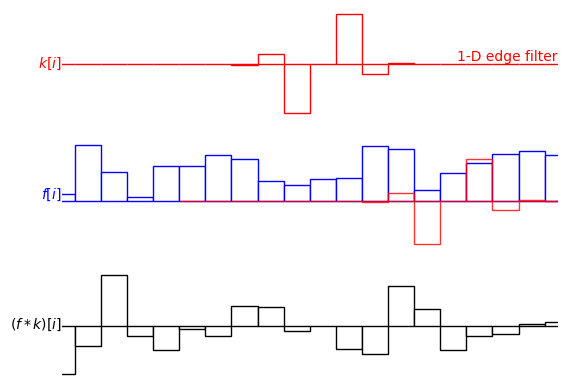
The convolution of two functions $f(x), w(x)$ is

\begin{align} (f * w)(x) = \int_{-\infty}^{\infty} f(t) \, w(x-t) \, dt \end{align}

or equivalently

\begin{align} (f * w)(x) = \int_{-\infty}^{\infty} f(x - t) \, w(x) \, dt \end{align}

Loosely, it’s a way of “mixing up” two functions. We sometimes refer to $w$ as a weighting function, or alternatively a kernel function.

Convolution has several very nice algebraic properties which we don’t need to get into. Read more here.

Computers are finite objects. So in general, we cannot evaluate integrals with infinitesimally small differentials $dt$ . Instead, we compute the discrete convolution using a sum

\begin{align} z[i] = \sum_{j=-\infty}^{\infty} x[i-j] \, w[j] \end{align}

Note that we also cannot evaluate sums over infinite domains. So we often work with finite kernels such that

\begin{align} z[i] = \sum_{j=-K}^{K} x[i-j] \, w[j] \end{align}

Implementing discrete convolutions¶

from math import floor

def discrete_convolution_1d(x, w, pad=0, stride=1):
    """ x is a numpy array of shape [N,]
        w is a numpy array of shape [k,]
    """
    N = x.shape[0]
    k = w.shape[0]
    out_size = floor((N + 2*pad - k) / stride + 1)

    if pad > 0:
        zeros = np.zeros(pad)
        x_pad = np.concatenate([zeros, x, zeros])
    else:
        x_pad = x

    result = []
    for ii in range(0, x_pad.shape[0] - k + 1, stride):
        result.append(
            np.sum(x_pad[ii:ii+k] * w[::-1]) # Reverse kernel matrix to compute convolution
        )
    return np.array(result)

x = np.array([1, 2, 3, 2, 2, 5, 2, 1], dtype=float)
w = np.array([-1, 0, 1]) # 1-D edge filter (first-order)

print(discrete_convolution_1d(x, w, pad=1, stride=1))
print(np.convolve(x, w, mode='same'))

[-2. -2.  0.  1. -3.  0.  4.  2.]
[-2. -2.  0.  1. -3.  0.  4.  2.]

def discrete_convolution_2d(x, w, pad=0, stride=1):
    N1, N2 = x.shape
    k1, k2 = w.shape

    if pad > 0:
        x_pad = np.zeros([N1+2*pad, N2+2*pad])
        x_pad[pad:-pad, pad:-pad] = x
    else:
        x_pad = x

    o1 = floor((N1 + 2*pad - k1) / stride + 1)
    o2 = floor((N2 + 2*pad - k2) / stride + 1)

    result = np.zeros([o1, o2])
    for i1, j1 in enumerate(range(0, x_pad.shape[0] - k1 + 1, stride)):
        for i2, j2 in enumerate(range(0, x_pad.shape[1] - k2 + 1, stride)):
            result[i1, i2] = np.sum(
                x_pad[j1:j1+k1, j2:j2+k2] * w[::-1, ::-1]
            )
    return result

x = np.random.randint(low=0, high=10, size=(5, 5)).astype(float)
print('For array x\n', x)
w = np.array([[-1, 0, 1], [-2, 0, 2], [-1, 0, 1]], dtype=float)

print('Our implementation:\n', discrete_convolution_2d(x, w, pad=1))
from scipy.signal import convolve2d
print('Scipy implementation:\n', convolve2d(x, w, mode='same'))

For array x
 [[9. 9. 7. 7. 2.]
 [6. 4. 8. 8. 9.]
 [1. 2. 0. 3. 7.]
 [3. 0. 4. 6. 9.]
 [0. 7. 9. 6. 3.]]
Our implementation:
 [[-22.   2.   0.   9.  22.]
 [-19.  -1.  -7.  -4.  26.]
 [ -8.  -1. -12. -20.  20.]
 [ -9. -10. -12. -11.  21.]
 [-14. -19.  -4.   7.  18.]]
Scipy implementation:
 [[-22.   2.   0.   9.  22.]
 [-19.  -1.  -7.  -4.  26.]
 [ -8.  -1. -12. -20.  20.]
 [ -9. -10. -12. -11.  21.]
 [-14. -19.  -4.   7.  18.]]

Speeding up discrete convolutions¶

# For loops are slow, how can we speed this up?
print(f"x is a float array of size {x.shape}")
print(f"A stride along dim 0 is {x.strides[0]} bytes: x[0] = {x[0]}")
print(f"A stride along dim 1 is {x.strides[1]} bytes: x[0,0] = {x[0, 0]}")

x is a float array of size (5, 5)
A stride along dim 0 is 40 bytes: x[0] = [9. 9. 7. 7. 2.]
A stride along dim 1 is 8 bytes: x[0,0] = 9.0

from numpy.lib.stride_tricks import as_strided
def fancy_convolution_2d(x, w, pad=0, stride=1, verbose=True):
    if verbose:
        print("Input x = \n", x)
    N1, N2 = x.shape
    k1, k2 = w.shape

    if pad > 0:
        x_pad = np.zeros([N1+2*pad, N2+2*pad])
        x_pad[pad:-pad, pad:-pad] = x
    else:
        x_pad = x

    o1 = floor((N1 + 2*pad - k1) / stride + 1)
    o2 = floor((N2 + 2*pad - k2) / stride + 1)
    
    # Instead of running nested for loops, add strides to the array to get windows equal to our kernel size
    x_stride = as_strided(
        x_pad,
        shape=(o1, # For each element in my output array along dim 0
               o2, # For each element in my output array along dim 1
               k1, # Give me a matrix with k1 rows
               k2),# Give me a matrix with k2 columns
        strides=(x_pad.strides[0], # Step in dim-0 is N1 x 8 bytes (move down a row)
                 x_pad.strides[1], # Step in dim-1 is 8 bytes (move over a column)
                 x_pad.strides[0], # Step in dim-2 is N1 x 8 bytes (move down a row)
                 x_pad.strides[1]) # Step in dim-3 is 8 bytes (move over a column)
    )
    
    if verbose:
        print(f"X has shape {x_stride.shape} and strides {x_stride.strides}")
        print(f"X[0, 0] = \n{x_stride[0, 0]}")
        print(f"X[1, 1] = \n{x_stride[1, 1]}")
        print()

    return np.einsum(
        'ijkl,kl->ij', x_stride, w[::-1, ::-1]
    )

print('Our implementation:\n', fancy_convolution_2d(x, w, pad=1))
print('Scipy implementation:\n', convolve2d(x, w, mode='same'))

Input x = 
 [[9. 9. 7. 7. 2.]
 [6. 4. 8. 8. 9.]
 [1. 2. 0. 3. 7.]
 [3. 0. 4. 6. 9.]
 [0. 7. 9. 6. 3.]]
X has shape (5, 5, 3, 3) and strides (56, 8, 56, 8)
X[0, 0] = 
[[0. 0. 0.]
 [0. 9. 9.]
 [0. 6. 4.]]
X[1, 1] = 
[[9. 9. 7.]
 [6. 4. 8.]
 [1. 2. 0.]]

Our implementation:
 [[-22.   2.   0.   9.  22.]
 [-19.  -1.  -7.  -4.  26.]
 [ -8.  -1. -12. -20.  20.]
 [ -9. -10. -12. -11.  21.]
 [-14. -19.  -4.   7.  18.]]
Scipy implementation:
 [[-22.   2.   0.   9.  22.]
 [-19.  -1.  -7.  -4.  26.]
 [ -8.  -1. -12. -20.  20.]
 [ -9. -10. -12. -11.  21.]
 [-14. -19.  -4.   7.  18.]]

from time import time

x = np.random.randint(low=0, high=10, size=(100, 100)).astype(float)

t = time()
basic = discrete_convolution_2d(x, w, pad=1)
print(f"Basic convolution took {time()-t:.06f} s")

t = time()
fancy = fancy_convolution_2d(x, w, pad=1, verbose=False)
print(f"Fancy convolution took {time()-t:.06f} s")

t = time()
theirs = convolve2d(x, w, mode='same')
print(f"Scipy convolution took {time()-t:.06f} s")

Basic convolution took 0.038687 s
Fancy convolution took 0.000414 s
Scipy convolution took 0.000303 s

Example: Gradient filter¶

from PIL import Image
import seaborn as sns
from matplotlib.colors import ListedColormap
img = np.array(Image.open('images/emmy.jpg').convert('L'))

from scipy.ndimage import convolve
filtered = convolve(img, w)

fig, ax = plt.subplots(1, 3, figsize=(8, 3))
ax[0].imshow(img, cmap='Greys_r')
sns.heatmap(data=w, annot=True, ax=ax[1], linecolor='black', linewidths=1, cmap=ListedColormap(['white']), cbar=False)
ax[1].set_aspect('equal')

ax[2].imshow(filtered, cmap='Greys_r')

for a in ax:
    a.axis('off')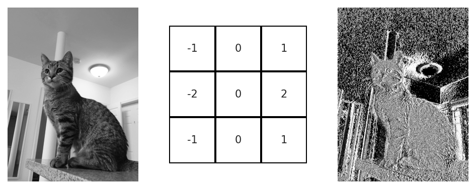

Example: edge detection (Sobel)¶

from PIL import Image
import seaborn as sns
from matplotlib.colors import ListedColormap
img = np.array(Image.open('images/emmy.jpg').convert('L'))

from scipy.ndimage import convolve
filtered_x = convolve(img, w)
filtered_y = convolve(img, w.T)

fig, ax = plt.subplots(2, 3, figsize=(8, 6))
ax[0,0].imshow(img, cmap='Greys_r')
ax[1,0].imshow(img, cmap='Greys_r')
sns.heatmap(data=w, annot=True, ax=ax[0,1], linecolor='black', linewidths=1, cmap=ListedColormap(['white']), cbar=False)
ax[0,1].set_aspect('equal')
sns.heatmap(data=w.T, annot=True, ax=ax[1,1], linecolor='black', linewidths=1, cmap=ListedColormap(['white']), cbar=False)
ax[1,1].set_aspect('equal')
ax[0,2].imshow(filtered_x, cmap='Greys_r')
ax[1,2].imshow(filtered_y, cmap='Greys_r')

for a in ax.flatten():
    a.axis('off')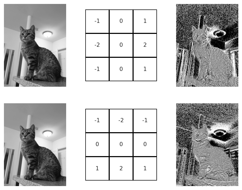

ax = plt.figure().gca()
ax.imshow(filtered_x**2 + filtered_y**2, cmap='Greys_r')
ax.axis('off');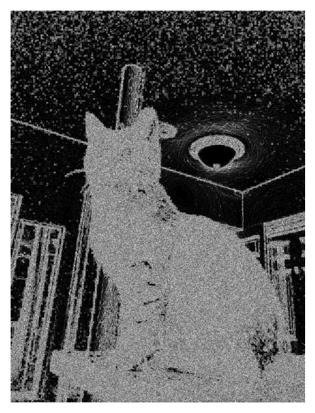

Image data often has multiple channels¶

from PIL import Image
import seaborn as sns
from matplotlib.colors import ListedColormap
img = np.array(Image.open('images/emmy.jpg').convert('RGB'))

fig, ax = plt.subplots(1, 4)
ax[0].imshow(img)
ax[1].imshow(img[..., 0], cmap='Reds_r')
ax[2].imshow(img[..., 1], cmap='Greens_r')
ax[3].imshow(img[..., 2], cmap='Blues_r')

for a in ax:
    a.axis('off')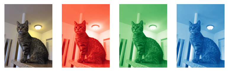

# Convolution that mixes channels
from numpy.lib.stride_tricks import as_strided
def multichannel_convolution_2d(x, w, pad=0, stride=1, verbose=True):
    """ X is a [N1, N2, 3] RGB image
        w is a [k1, k2, c1, c2] rank 4 tensor (a "matrix of matrices")
    """
    N1, N2, c = x.shape
    k1, k2, c_in, c_out = w.shape

    if pad > 0:
        x_pad = np.zeros([N1+2*pad, N2+2*pad, c])
        x_pad[pad:-pad, pad:-pad] = x
    else:
        x_pad = x

    o1 = floor((N1 + 2*pad - k1) / stride + 1)
    o2 = floor((N2 + 2*pad - k2) / stride + 1)
    
    # Instead of running nested for loops, add strides to the array to get windows equal to our kernel size
    x_stride = as_strided(
        x_pad,
        shape=(o1, # For each element in my output array along dim 0
               o2, # For each element in my output array along dim 1
               c,  # For each feature at that pixel position
               k1, # Give me a matrix with k1 rows
               k2), # Give me a matrix with k2 columns
        strides=(x_pad.strides[0], # Step in dim-0 is N2 x c bytes (x is of type uint8)
                 x_pad.strides[1], # Step in dim-1 is c bytes
                 x_pad.strides[2], # Step in dim-2 is 1 byte (uint8)
                 x_pad.strides[0], # Step in dim-3 is N2 x c bytes (move down one row)
                 x_pad.strides[1]) # Step in dim-4 is c bytes (move over one column)
    )
    
    return np.einsum(
        'ijckl,klcd->ijd', x_stride, w[::-1, ::-1]
    )

w_array = np.zeros([*w.shape, 3, 6])
w_array[:, :, 0, 0] = w
w_array[:, :, 0, 1] = w.T
w_array[:, :, 1, 2] = w
w_array[:, :, 1, 3] = w.T
w_array[:, :, 2, 4] = w
w_array[:, :, 2, 5] = w.T

out = multichannel_convolution_2d(img, w_array, stride=1, pad=1)
print(out.shape)

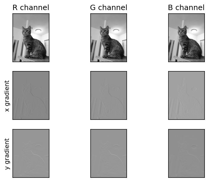
fig, ax = plt.subplots(3, 3)
for ii in range(3):
    ax[0, ii].imshow(img[..., 0], cmap='Greys_r')
    ax[1, ii].imshow(out[..., ii*2], cmap='Greys_r')
    ax[2, ii].imshow(out[..., ii*2 + 1], cmap='Greys_r')


ax[0,0].set_title('R channel')
ax[0,1].set_title('G channel')
ax[0,2].set_title('B channel')

ax[1,0].set_ylabel('x gradient')
ax[2,0].set_ylabel('y gradient')

for a in ax.flatten():
    a.set(xticks=[], yticks=[])
    a.grid(False)

(1674, 1256, 6)

ax = plt.figure().gca()
edge = np.linalg.norm(out, axis=2)
ax.imshow(edge, cmap='Greys_r')
ax.axis('off')

(-0.5, 1255.5, 1673.5, -0.5)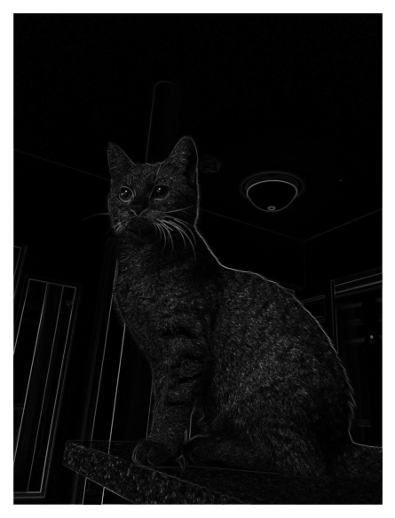

from torch.nn.functional import conv2d

img_torch = torch.FloatTensor(img).permute(2, 0, 1)[None] # Torch uses channels-first by default and requires a batch dimension
w_torch = torch.FloatTensor(w_array).permute(3, 2, 0, 1) # Channels-first by default, see documentation

out = conv2d(input=img_torch,
             weight=w_torch,
             stride=1, padding='same')

fig, ax = plt.subplots(3, 3)
for ii in range(3):
    ax[0, ii].imshow(img[..., 0], cmap='Greys_r')
    ax[1, ii].imshow(out[0, ii*2], cmap='Greys_r')
    ax[2, ii].imshow(out[0, ii*2 + 1], cmap='Greys_r')


ax[0,0].set_title('R channel')
ax[0,1].set_title('G channel')
ax[0,2].set_title('B channel')

ax[1,0].set_ylabel('x gradient')
ax[2,0].set_ylabel('y gradient')

for a in ax.flatten():
    a.set(xticks=[], yticks=[])
    a.grid(False)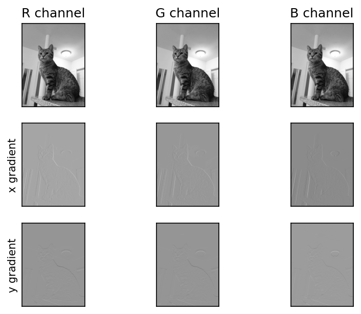

ax = plt.figure().gca()
edge = np.linalg.norm(out, axis=(0,1))
ax.imshow(edge, cmap='Greys_r')
ax.axis('off')

(-0.5, 1255.5, 1673.5, -0.5)

torch.nn.functional.conv2d?

Docstring:
conv2d(input, weight, bias=None, stride=1, padding=0, dilation=1, groups=1) -> Tensor

Applies a 2D convolution over an input image composed of several input
planes.

This operator supports :ref:`TensorFloat32<tf32_on_ampere>`.

See :class:`~torch.nn.Conv2d` for details and output shape.

Note:
    In some circumstances when given tensors on a CUDA device and using CuDNN, this operator may select a nondeterministic algorithm to increase performance. If this is undesirable, you can try to make the operation deterministic (potentially at a performance cost) by setting ``torch.backends.cudnn.deterministic = True``. See :doc:`/notes/randomness` for more information.

Note:
    This operator supports complex data types i.e. ``complex32, complex64, complex128``.


Args:
    input: input tensor of shape :math:`(\text{minibatch} , \text{in\_channels} , iH , iW)`
    weight: filters of shape :math:`(\text{out\_channels} , \frac{\text{in\_channels}}{\text{groups}} , kH , kW)`
    bias: optional bias tensor of shape :math:`(\text{out\_channels})`. Default: ``None``
    stride: the stride of the convolving kernel. Can be a single number or a
      tuple `(sH, sW)`. Default: 1
    padding: implicit paddings on both sides of the input. Can be a string {'valid', 'same'},
      single number or a tuple `(padH, padW)`. Default: 0
      ``padding='valid'`` is the same as no padding. ``padding='same'`` pads
      the input so the output has the same shape as the input. However, this mode
      doesn't support any stride values other than 1.

      .. warning::
          For ``padding='same'``, if the ``weight`` is even-length and
          ``dilation`` is odd in any dimension, a full :func:`pad` operation
          may be needed internally. Lowering performance.

    dilation: the spacing between kernel elements. Can be a single number or
      a tuple `(dH, dW)`. Default: 1
    groups: split input into groups, both :math:`\text{in\_channels}` and :math:`\text{out\_channels}`
      should be divisible by the number of groups. Default: 1

Examples::

    >>> # With square kernels and equal stride
    >>> filters = torch.randn(8, 4, 3, 3)
    >>> inputs = torch.randn(1, 4, 5, 5)
    >>> F.conv2d(inputs, filters, padding=1)
Type:      builtin_function_or_method