PyTorch Autograd
!pip install torchviz torch==2.13.0Requirement already satisfied: torchviz in /Users/jcolen/miniconda3/envs/pytorch/lib/python3.10/site-packages (0.0.3)
Requirement already satisfied: torch==2.13.0 in /Users/jcolen/miniconda3/envs/pytorch/lib/python3.10/site-packages (2.13.0)
Requirement already satisfied: filelock in /Users/jcolen/miniconda3/envs/pytorch/lib/python3.10/site-packages (from torch==2.13.0) (4.0.1)
Requirement already satisfied: typing-extensions>=4.10.0 in /Users/jcolen/miniconda3/envs/pytorch/lib/python3.10/site-packages (from torch==2.13.0) (4.16.0)
Requirement already satisfied: setuptools>=77.0.3 in /Users/jcolen/miniconda3/envs/pytorch/lib/python3.10/site-packages (from torch==2.13.0) (84.0.0)
Requirement already satisfied: sympy>=1.13.3 in /Users/jcolen/miniconda3/envs/pytorch/lib/python3.10/site-packages (from torch==2.13.0) (1.14.0)
Requirement already satisfied: networkx>=2.5.1 in /Users/jcolen/miniconda3/envs/pytorch/lib/python3.10/site-packages (from torch==2.13.0) (3.4.2)
Requirement already satisfied: jinja2 in /Users/jcolen/miniconda3/envs/pytorch/lib/python3.10/site-packages (from torch==2.13.0) (3.1.6)
Requirement already satisfied: fsspec>=0.8.5 in /Users/jcolen/miniconda3/envs/pytorch/lib/python3.10/site-packages (from torch==2.13.0) (2026.9.0)
Requirement already satisfied: graphviz in /Users/jcolen/miniconda3/envs/pytorch/lib/python3.10/site-packages (from torchviz) (0.21)
Requirement already satisfied: mpmath<1.4,>=1.1.0 in /Users/jcolen/miniconda3/envs/pytorch/lib/python3.10/site-packages (from sympy>=1.13.3->torch==2.13.0) (1.3.0)
Requirement already satisfied: MarkupSafe>=2.0 in /Users/jcolen/miniconda3/envs/pytorch/lib/python3.10/site-packages (from jinja2->torch==2.13.0) (3.0.3)
%matplotlib inline
import numpy as np
import matplotlib.pyplot as plt
import seaborn as sns
import pandas as pd
import torch
plt.rcParams['xtick.direction'] = 'in'
plt.rcParams['ytick.direction'] = 'in'
plt.rcParams['axes.grid'] = True
plt.rcParams['axes.axisbelow'] = True
plt.rcParams['figure.dpi'] = 150

# Check available hardware
if torch.cuda.is_available():
    device = torch.device('cuda')
    print(f'GPU is available, using {device}')
elif torch.mps.is_available():
    device = torch.device('mps')
    print(f'Apple Metal Performance Shaders framework is available, using {device}')
else:
    device = torch.device('cpu')
    print(f'Hardware acceleration not available, using {device}')

tkwargs = {'dtype': torch.float, 'device': device} # For tensor initialization
Apple Metal Performance Shaders framework is available, using mps
import os
os.environ['PATH'] = f'/opt/homebrew/bin/:{os.environ["PATH"]}'
Concepts of PyTorch Autograd
requires_gradenables gradient trackinggrad_fnenables gradient backpropagationis_leafdefines whether a tensor is a leaf tensor
x = torch.tensor([2., 3.], requires_grad=True, **tkwargs)
y = torch.tensor([1., 2.], requires_grad=True, **tkwargs)
c = torch.tensor([3., 4.], requires_grad=True, **tkwargs)

print(f"x: {x}\ny: {y}\nc: {c}")
x: tensor([2., 3.], device='mps:0', requires_grad=True)
y: tensor([1., 2.], device='mps:0', requires_grad=True)
c: tensor([3., 4.], device='mps:0', requires_grad=True)
z = x * y + c
print(f"z: {z}")

loss = torch.mean(torch.rand(z.shape, **tkwargs) - z).pow(2)
print(f"loss: {loss}")
loss
z: tensor([ 5., 10.], device='mps:0', grad_fn=<AddBackward0>)
loss: 46.59133529663086
tensor(46.5913, device='mps:0', grad_fn=<PowBackward0>)A leaf tensor is a tensor that does not have a grad_fn. It is not further differentiable. It is typically a network parameter that has been initialized by the user, and does not originate as the result of some computation.
A root tensor is the start of what we will call the computational graph. It is what we call backward() from to begin gradient backpropagation.
for name, tensor in zip(['x', 'y', 'c', 'z', 'loss'], [x, y, c, z, loss]):
    print(f"Is {name} a leaf tensor: {tensor.is_leaf}\t{tensor}")
Is x a leaf tensor: True tensor([2., 3.], device='mps:0', requires_grad=True)
Is y a leaf tensor: True tensor([1., 2.], device='mps:0', requires_grad=True)
Is c a leaf tensor: True tensor([3., 4.], device='mps:0', requires_grad=True)
Is z a leaf tensor: False tensor([ 5., 10.], device='mps:0', grad_fn=<AddBackward0>)
Is loss a leaf tensor: False 46.59133529663086
Break the above down into elementary computations
# Create a tensor and set requires_grad=True to track its gradients
x = torch.tensor([2.0, 3.0], requires_grad=True, **tkwargs)
y = torch.tensor([1.0, 2.0], requires_grad=True, **tkwargs)
c = torch.tensor([3.0, 4.0], requires_grad=True, **tkwargs)

# step 1: multiply x and y
r1 = torch.mul(x, y)
# step 2: add r1 with c
w = torch.add(r1, c)
# step 3: Take mean of w
z = torch.mean(w)

for name, tensor in zip(['x', 'y', 'c', 'r1', 'w', 'z'], [x, y, c, r1, w, z]):
    print(f"Is {name} a leaf tensor: {tensor.is_leaf}\t{tensor}")
Is x a leaf tensor: True	tensor([2., 3.], device='mps:0', requires_grad=True)
Is y a leaf tensor: True	tensor([1., 2.], device='mps:0', requires_grad=True)
Is c a leaf tensor: True	tensor([3., 4.], device='mps:0', requires_grad=True)
Is r1 a leaf tensor: False	tensor([2., 6.], device='mps:0', grad_fn=<MulBackward0>)
Is w a leaf tensor: False	tensor([ 5., 10.], device='mps:0', grad_fn=<AddBackward0>)
Is z a leaf tensor: False	7.5
z.backward(retain_graph=True)
for name, tensor in zip(['x', 'y', 'c'], [x, y, c]):
    print(f'gradient of {name}: {tensor.grad.tolist()}')
gradient of x: [0.5, 1.0]
gradient of y: [1.0, 1.5]
gradient of c: [0.5, 0.5]
z.backward(retain_graph=True)# An intermediate non-leaf variable - does it have a grad attribute?
r1.gradimport torchviz
torchviz.make_dot(z, {'x': x, 'y': y, 'c': c, 'z': z, 'w': w, 'r1': r1}, show_attrs=True)a = torch.tensor([2., 3.], requires_grad=True, **tkwargs)
b = torch.tensor([6., 4.], requires_grad=True, **tkwargs)
Q = 3 * a**3 - b**2
print(Q.shape)torch.Size([2])
We can call backward(gradient="something") which defines the running gradient with respect to each output tensor element.
gradient = torch.tensor([1., 1.], **tkwargs)
Q.retain_grad()
Q.backward(gradient=gradient)
# Check that the gradients equal our ground truth estimate
print(9*a**2 == a.grad)
print(-2*b == b.grad)tensor([True, True], device='mps:0')
tensor([True, True], device='mps:0')
torchviz.make_dot(Q, params={'a': a, 'b': b, 'Q': Q})w = torch.tensor(1., requires_grad=True)
b = torch.tensor(0., requires_grad=True)
x = torch.tensor([0.5])
y = torch.tensor([6.8])
z = w * x + b
loss = (y - z).pow(2).sum()
loss.backward()
print(f'dL/dw = {w.grad}, should be {2*x*(z - y)}')
print(f'dL/db = {b.grad}, should be {2*(z - y)}')dL/dw = -6.300000190734863, should be tensor([-6.3000], grad_fn=<MulBackward0>)
dL/db = -12.600000381469727, should be tensor([-12.6000], grad_fn=<MulBackward0>)
torchviz.make_dot(loss, params={'w': w, 'b': b, 'loss': loss, 'x': x, 'y': y, 'z': z})Using this in a torch neural network
import torch
import torch.nn as nn
import torch.nn.functional as F

class NN(nn.Module):
    def __init__(self):
        super().__init__()

        self.fc1 = nn.Linear(1, 4)
        self.fc2 = nn.Linear(4, 1)

    def forward(self, x):
        x = F.relu(self.fc1(x))
        x = F.tanh(self.fc2(x))
        return x

model = NN()
inputs = torch.rand(1)
outputs = model(inputs)

print(f"Inputs:  {inputs}")
print(f"Outputs: {outputs}")
Inputs: tensor([0.0331])
Outputs: tensor([0.2693], grad_fn=<TanhBackward0>)
import torchviz
torchviz.make_dot(outputs, {'inputs': inputs, 'outputs': outputs})Comparing different ways to compute gradients
Consider the sigmoid activation function below. Its computational graph will break it down into elementary computations
def sigmoid(x):
    return 1 / (1. + torch.exp(-x))

x = torch.tensor(1., requires_grad=True)
s = sigmoid(x)

torchviz.make_dot(s, params={'x': x, 's': s})This is a lot of operations for a single activation. Backprop has to handle at least four compositions
def grad_sigmoid_analytic(x):
    """ We know this is the answer from our in-class derivation
    """
    z = sigmoid(x)
    return z * (1 - z)

def grad_sigmoid_pytorch(x):
    """ The easy way to compute gradients
    """
    z = sigmoid(x)
    z.backward()
    return x.grad

def grad_sigmoid_reverse_mode(x):
    """ Manually breaking down the computation into smaller steps
    """
    a = -x
    b = np.exp(a)
    c = 1 + b
    d = 1 / c

    dddc = -1. / c**2
    dddb = dddc * 1
    ddda = dddb * np.exp(a)
    dddx = -ddda

    return dddx

def grad_sigmoid_forward_mode(x):
    """ Another option is to compute gradients during the forward pass """
    a = -x
    dadx = -1.

    b = np.exp(a)
    dbda = np.exp(a)
    dbdx = dbda * dadx

    c = 1 + b
    dcdb = 1.
    dcdx = dcdb * dbdx

    d = 1/c
    dddc = -1. / c**2
    dddx = dddc * dcdx

    return dddx

x = torch.tensor(1., requires_grad=True)
print(f"Analytical derivative: {grad_sigmoid_analytic(x)}", flush=True)
print(f"PyTorch Autograd: {grad_sigmoid_pytorch(x)}")
print(f"Manual Reverse-Mode: {grad_sigmoid_reverse_mode(x.detach().numpy())}")
print(f"Manual Forward-Mode: {grad_sigmoid_forward_mode(x.detach().numpy())}")
Analytical derivative: 0.1966119259595871
PyTorch Autograd: 0.1966119408607483
Manual Reverse-Mode: 0.19661197066307068
Manual Forward-Mode: 0.19661197066307068
Manually coding a 1-hidden layer NN
def sigmoid(x):
    return 1. / (1. + torch.exp(-x))

def grad_sigmoid(z):
    return z * (1 - z)

def relu(x):
    return torch.maximum(x, torch.tensor(0.))

def grad_relu(x):
    return torch.where(x > 0, torch.tensor(1.), torch.tensor(0.))

def forward(x, w1, w2):
    z1 = x @ w1.T # [B, I] x [I, H]
    h1 = relu(z1)

    z2 = h1 @ w2.T # [B, H] x [H, O]
    h2 = sigmoid(z2)

    return h2, z1, h1, z1

def backward_autograd(x, w1, w2, y):
    x.requires_grad_(True)
    w1.requires_grad_(True)
    w2.requires_grad_(True)

    y_pred, _, _, _ = forward(x, w1, w2)
    loss = (y_pred - y).pow(2).mean()
    loss.backward()

    return w1.grad, w2.grad

def backward_manual(x, w1, w2, y):
    h2, z2, h1, z1 = forward(x, w1, w2)
    loss = (h2 - y).pow(2).mean()

    dloss_dh2 = 2 * (h2 - y) * y.numel() # [B, O]
    dloss_dz2 = dloss_dh2 * grad_sigmoid(h2) # [B, O]

    dloss_dw2 = dloss_dz2.T @ h1 # [O, B] x [B, H]

    dloss_dh1 = dloss_dz2 @ w2 # [B, O] x [O, H]
    dloss_dz1 = dloss_dh1 * grad_relu(z1) # [B, H]

    dloss_dw1 = dloss_dz1.T @ x # [H, B] x [B, I]

    return dloss_dw1, dloss_dw2


x = torch.rand([1, 2]) #[B, I]
w1 = torch.rand([4, 2]) #[H, I]
w2 = torch.rand([1, 4]) #[O, H]
y = torch.rand(1) #[]

print("With autograd:", flush=True)
w1_grad, w2_grad = backward_autograd(x, w1, w2, y)
print(f'w1_grad = {w1_grad}')
print(f'w2_grad = {w2_grad}')

print('-------------')
print('Manually (reverse-mode):')
w1_grad, w2_grad = backward_manual(x, w1, w2, y)
print(f'w1_grad = {w1_grad}')
print(f'w2_grad = {w2_grad}', flush=True)
With autograd:
w1_grad = tensor([[0.0026, 0.0051],
        [0.0069, 0.0135],
        [0.0044, 0.0086],
        [0.0034, 0.0068]])
w2_grad = tensor([[0.0079, 0.0081, 0.0210, 0.0165]])
-------------
Manually (reverse-mode):
w1_grad = tensor([[0.0026, 0.0051],
        [0.0069, 0.0135],
        [0.0044, 0.0086],
        [0.0034, 0.0068]], grad_fn=<MmBackward0>)
w2_grad = tensor([[0.0079, 0.0081, 0.0210, 0.0165]], grad_fn=<MmBackward0>)
Note that we’re doing this “reverse-mode automatic differentiation” by starting with derivatives from the loss and propagating backward.
That is, we’re performing the above operation from left to right. For a single example, the size of each tensor is
Thus, the total number of operations here is
Another way to do it would be to do “forward-mode automatic differentiation,” which performs the above operation from right to left.
Here, the total number of operations is
Suppose we have a contracting computation, i.e. . Then , and we expect reverse-mode automatic differentiation to be more efficient than forward-mode. Typically, if , reverse-mode is more efficient, while if , forward-mode is more efficient. The latter is a less common situation, and in fact PyTorch’s forward-mode autodiff is still in beta.
Autograd can compute derivatives of functions for us
x = torch.linspace(0, 2.*torch.pi, 100, requires_grad=True)
z = torch.sin(x)
dz_dx = torch.autograd.grad(
    outputs=z,
    inputs=x,
    grad_outputs=torch.ones_like(z), # dz/dz = 1
    create_graph=True # We want to create a computation graph
)[0]
ax = plt.figure().gca()
ax.plot(x.detach().cpu().numpy(), z.detach().cpu().numpy(), label='f(x) = sin(x)')
ax.plot(x.detach().cpu().numpy(), dz_dx.detach().cpu().numpy(), label='df/dx')
ax.plot(x.detach().cpu().numpy(), torch.cos(x).detach().cpu().numpy(), label='cos(x)', linestyle='--')
ax.legend();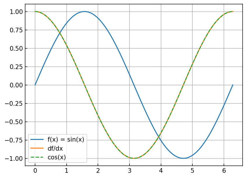
This framework extends pretty far, for example to 2D images
x = torch.linspace(0., 2. * torch.pi, 100, requires_grad=False)
y = torch.linspace(0., 2. * torch.pi, 100, requires_grad=False)

X, Y = torch.meshgrid(x, y, indexing='xy')
X.requires_grad = True
Y.requires_grad = True

V = X + Y
V.retain_grad()

Z = torch.sin(V)
Z.retain_grad()

Z.backward(gradient=torch.ones_like(Z))
plt.rcParams['image.origin'] = 'lower'
with torch.no_grad():
fig, ax = plt.subplots(1, 3, sharex=True, sharey=True)
ax[0].pcolormesh(X, Y, Z, cmap='bwr', vmin=-1, vmax=1)
ax[0].set_title('$f(x, y) = \\sin(x + y)$')
dz_dx = X.grad
dz_dy = Y.grad
grad_Z = torch.sqrt(dz_dx**2 + dz_dy**2)
skip = 5
ax[1].pcolormesh(X, Y, grad_Z, cmap='bwr', vmin=-1, vmax=1)
ax[1].quiver(X[::skip, ::skip], Y[::skip, ::skip], dz_dx[::skip, ::skip], dz_dy[::skip, ::skip])
ax[1].set_title('$\\nabla f = \\cos(x + y) (\\hat{x} + \\hat{y})$')
ax[2].pcolormesh(X, Y, Z**2 + 0.5 * grad_Z**2, cmap='bwr', vmin=-1, vmax=1)
ax[2].set_title('$f^2 + \\frac{1}{2} |\\nabla f|^2$')
for a in ax.flatten():
a.set(aspect='equal')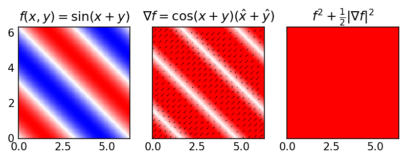
with torch.no_grad():
    fig, ax = plt.subplots(2, 2, sharex=True, sharey=True)

    ax[0,0].pcolormesh(X, Y, V, cmap='magma')
    ax[0,0].set_title('$V = X + Y$')

    ax[0,1].pcolormesh(X, Y, Z, cmap='bwr', vmin=-1, vmax=1)
    ax[0,1].set_title('$f(V) = \\sin(V)$')

    dz_dv = V.grad
    ax[1,0].pcolormesh(X, Y, dz_dv, cmap='bwr', vmin=-1, vmax=1)
    ax[1,0].set_title('$\\nabla_V f(V) = \\cos(V)$')

    ax[1,1].pcolormesh(X, Y, Z**2 + dz_dv**2, cmap='bwr', vmin=-1, vmax=1)
    ax[1,1].set_title('$f(V)^2 + |\\nabla_V f(V)|^2 = 1$')

    for a in ax.flatten():
        a.set(aspect='equal')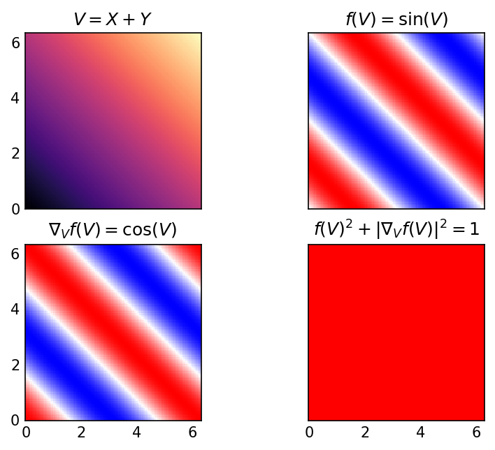
torchviz.make_dot(Z, params={'X': X, 'Y': Y, 'V': V, 'Z': Z})